

In intelligent manufacturing logistics systems, the continuous and stable operation of AGVs (Automated Guided Vehicles) relies directly on the scientific selection of the battery system. A well-designed battery solution not only guarantees uninterrupted operation within the production takt time, but also significantly reduces total life-cycle cost, minimizes charging downtime, and extends battery service life.
Based on real project data (takt time 15 JPH, rated power 6000 W, rated voltage 48 V), this article systematically presents a complete engineering methodology for AGV battery selection, covering the full process from theoretical modeling to practical implementation. The objective is to provide engineers with a reusable and verifiable technical framework.
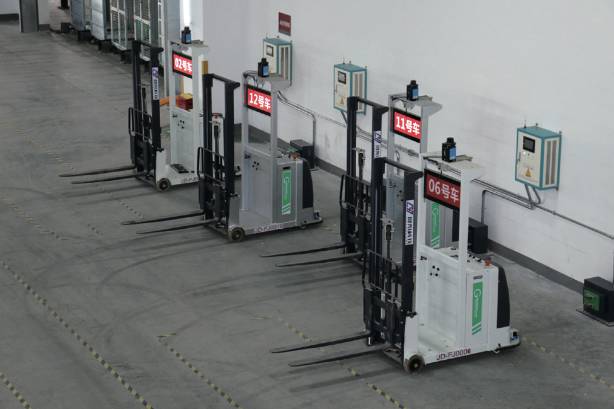
Engineering Warning
AGV battery selection is not a simple capacity-matching exercise. It is a system-level engineering task that integrates mechanical dynamics, electrochemistry, thermodynamics, and production scheduling. Improper selection may lead to unexpected power loss during operation, or excessive capacity redundancy that increases cost without improving performance. Industry statistics indicate that approximately 30 percent of AGV operation and maintenance issues originate from incorrect battery selection during the initial design phase.
1. Physical Modeling of AGV Energy Consumption
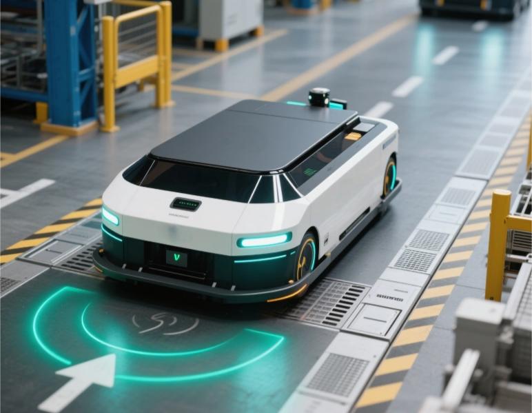
The total energy consumption of an AGV is equal to the combined energy consumption of all subsystems and must include an appropriate safety margin. The following derivation is based on classical mechanics and fundamental electrical principles.
1.1 Traction Force Calculation: The Source of Mechanical Energy Consumption
During motion, an AGV must overcome rolling resistance from the ground. The required traction force is calculated as:
F = (M_load + M_carrier + M_vehicle) × g × μ
Where
F is the traction force, in newtons
M_load is the payload mass, 1200 kg
M_carrier is the carrier mass, 0 kg, as the AGV has an integrated load structure
M_vehicle is the AGV self-weight, 1600 kg
g is the gravitational acceleration, taken as 9.8 m/s²
μ is the rolling friction coefficient, selected as 0.06 for a smooth concrete floor
Project calculation example
F = (1200 + 0 + 1600) × 9.8 × 0.06 ≈ 1646.4 N
Engineering note
The friction coefficient must be selected according to actual floor conditions. Typical values are 0.05 to 0.07 for smooth concrete floors, 0.04 to 0.06 for epoxy floors, and 0.08 to 0.12 for rough surfaces. A deviation of 10 percent in μ will directly result in a similar deviation in subsequent power calculations.
1.2 Operating Power Calculation: Conversion from Mechanical Energy to Electrical Power
The operating power required during steady motion is calculated as:
P_run = F × v / 60
Where
P_run is the operating power, in watts
v is the AGV travel speed, 30 meters per minute
Loaded condition
P_run = 1646.4 × 30 / 60 ≈ 823.2 W
Unloaded condition
When the payload is zero, the traction force becomes:
F_unloaded = 1600 × 9.8 × 0.06 ≈ 940.8 N
P_unloaded = 940.8 × 30 / 60 ≈ 470.4 W
1.3 Operating Current Calculation
The operating current is derived using the basic electrical relationship:
I = P / V
Where
I is the operating current, in amperes
V is the rated DC voltage of the AGV, 48 V
Loaded condition
I_loaded = 823.2 / 48 ≈ 17.15 A
Unloaded condition
I_unloaded = 470.4 / 48 ≈ 9.8 A
Rated current verification
The rated power of the AGV is 6000 W. The corresponding rated current is:
I_rated = 6000 / 48 = 125 A
This value is significantly higher than the actual operating current, indicating sufficient design margin to accommodate transient high-power demands such as startup, acceleration, and lifting operations.
1.4 Integrated Energy Consumption of Multiple Subsystems
1.4.1 Drive System Energy Consumption per Cycle
The travel time for a single run is determined by distance and speed.
t_run = travel distance / travel speed
t_run = 30 meters / 30 meters per minute = 1 minute
Energy consumption for one run is calculated as:
Q_run = I × t_run / 60
Loaded condition
Q_run = 17.15 × 1 / 60 ≈ 0.2858 Ah
Unloaded condition
Q_run = 9.8 × 1 / 60 ≈ 0.1633 Ah
1.4.2 Control System Energy Consumption
The control system power consumption is 50 W at 24 V. The energy consumption per cycle is:
Q_control = (50 / 24) × 1 ≈ 2.0833 Ah
1.4.3 Lifting Mechanism Energy Consumption
The lifting mechanism power is 2000 W. The lifting operation time per cycle is 3 minutes. The system voltage is 48 V.
Q_lift = (2000 / 48) × 3 / 60 ≈ 2.0833 Ah
1.4.4 Total Energy Consumption and Safety Factor
The total energy consumption per cycle is calculated as:
Q_total = (Q_run + Q_control + Q_lift) × k_safety
The safety factor k_safety is typically selected between 1.2 and 1.5. In this project, a value of 1.2 is applied.
Loaded condition
Q_total = (0.2858 + 2.0833 + 2.0833) × 1.2 ≈ 5.337 Ah
Unloaded condition
Q_total = (0.1633 + 2.0833 + 2.0833) × 1.2 ≈ 5.195 Ah
Engineering experience
For flat indoor environments, a safety factor of 1.2 is sufficient. For applications involving slopes up to 5 degrees or frequent start-stop cycles, values between 1.3 and 1.4 are recommended. Outdoor or harsh environments typically require values between 1.4 and 1.5.
2. Engineering Method for Battery Capacity Selection

2.1 Determination of Battery Utilization Rate
Battery utilization rate, denoted as η, accounts for discharge depth limits, aging degradation, and temperature effects. For lithium batteries, the maximum recommended depth of discharge is typically 80 percent. Considering a three-year service life and environmental factors, a utilization rate of 80 percent is adopted in this project.
The required nominal battery capacity is calculated as:
C_required = Q_total / η
Project example
C_required = 5.337 / 0.8 ≈ 6.671 Ah
2.2 Engineering Rounding Principles for Battery Capacity
Theoretical calculations must be aligned with commercially available battery specifications. The following principles are applied:
Capacity should always be rounded upward to ensure sufficient margin
Standard market capacities should be prioritized
Voltage matching must be ensured, with a 48 V system typically formed by four 12 V battery modules in series
Final selection
A 120 Ah, 48 V lithium battery system is selected.
Theoretical supported number of cycles:
120 / 5.337 ≈ 22 cycles
At a takt time of 15 JPH, the continuous operating time is:
22 / 15 ≈ 1.47 hours
This configuration provides sufficient margin to accommodate future payload increases, battery aging, and abnormal operating conditions.
2.3 Comparison of Battery Technologies
Lead-acid batteries typically offer low energy density and limited cycle life, while lithium iron phosphate batteries provide significantly higher energy density, longer service life, and faster charging capability.
From an engineering and life-cycle cost perspective, lithium iron phosphate batteries are better suited for AGV applications, especially in systems requiring opportunity charging and high availability.
The selected lithium battery supports a maximum charging rate of 2C, which provides a critical technical basis for the design of fast-charging systems.
3. Charging System Design and Calculation

3.1 Selection of Charging Current
To balance charging speed and battery lifespan, a charging rate of 1C is selected.
I_charge = 120 A
The decision to use 1C instead of 2C charging is based on the following considerations:
Charging time remains within acceptable limits
Battery aging is reduced
Impact on the factory power grid is minimized
Charging equipment cost is lower
3.2 Accurate Charging Time Calculation
Charging time is calculated using the following relationship:
t_charge = Q_required / (I_charge × n_stations) × 60
Where
Q_required is the energy required per cycle, 5.337 Ah
I_charge is the charging current, 120 A
n_stations is the number of charging stations, 2
Project calculation
t_charge ≈ 1.33 minutes
This indicates that after completing one operation cycle of approximately 3 minutes, the AGV requires only about 1.33 minutes of charging to replenish the consumed energy, fully satisfying the 15 JPH takt requirement.
3.3 Optimization of Charging Station Quantity
The number of charging stations must be determined based on AGV quantity, charging time, operating time, available space, and cost.
For a single charging station, the maximum number of supported cycles per hour is:
60 / (t_charge + t_operation)
60 / (1.33 + 3) ≈ 13.85 cycles per hour
With two charging stations, the total service capacity becomes approximately 27.7 cycles per hour.
The maximum number of AGVs supported is:
27.7 / 15 ≈ 1.85
This result is rounded up to 2 AGVs.
Conclusion
Two charging stations are sufficient to support continuous operation of two AGVs. For larger fleets, additional charging stations or higher charging currents are required.
4. Key Technical Risks and Engineering Countermeasures
Key risks include capacity calculation deviation, charging safety, temperature impact, and battery aging.
Recommended countermeasures include real-world energy consumption testing, conservative capacity margin design, use of batteries with integrated BMS, multi-level charging protection, environmental monitoring, and full life-cycle battery data tracking.
5. Engineering Validation and Optimization Recommendations
5.1 Technical Validation
The following tests are recommended to verify the feasibility of the selected solution:
Static capacity testing under controlled discharge conditions
Continuous operation testing at 15 JPH for eight hours
Charging efficiency testing to verify efficiency above 90 percent
5.2 Continuous Optimization Recommendations
An intelligent energy management system can be deployed to collect real-time energy and battery data, dynamically optimize charging strategies, and predict battery health status.
Charging tasks should be integrated into the AGV scheduling system to achieve load balancing across charging stations and prioritize low-state-of-charge vehicles.
In the long term, hybrid energy storage solutions combining supercapacitors and lithium batteries, wireless charging technologies, and AI-based path optimization algorithms can be considered to further improve system efficiency.
Conclusion
AGV battery selection is a multidisciplinary system engineering task. Based on real project data, this article establishes a complete technical pathway covering energy consumption modeling, capacity calculation, charging system configuration, and risk mitigation.
The final solution, consisting of a 120 Ah, 48 V lithium battery system and two 120 A charging stations, has been validated through engineering calculations and is fully capable of supporting continuous AGV operation at a takt time of 15 JPH.
For AGV system engineers, mastering this structured and scientific selection methodology not only ensures equipment reliability, but also improves overall logistics efficiency and economic performance, providing solid technical support for the successful deployment of intelligent manufacturing systems.


